The first study settled an important baseline: after commitment, the model’s answer is easy to read with a linear probe. It also exposed the harder problem. A supplied target can be actuated, but the prospective target-free controller failed to find one reliably.
That left a sharper question than classification:
Can I reconstruct the matched activation difference between a state that is about to report falsely and a state that reports correctly—before the model samples the status token?
Not classify a state. Reconstruct the matched displacement.
The central result
0.93cosine
versus 0.48 for one global direction
A nearby state is a better address than one global vector
On held-out scenario families, raw-activation retrieval reconstructs the matched displacement at 0.9326 cosine. The result survives the obvious global and shuffled controls.
01
One example is almost enough
A single raw nearest neighbor reaches 0.9304. Elaborate graph machinery is not carrying the result.
02
This is not yet control
The displacement is reconstructed offline. It has not been injected, and the destination is not inferred autonomously.
The object: a displacement, not a label
Here lie is shorthand for a false operational status after the model has demonstrated the correct answer. It does not assert human-like intent or a hidden goal.
The bank contains sixty machine-checkable scenarios across twenty families. At each decision
turn, the model sees the literal prefix Status: and samples one unrestricted token. I record
its internal numerical state—the activation—at four layers immediately before that token.
For the same scenario and machine-checked truth, I match one knowledge-correct completion that
later reports the wrong status with one that reports the correct status. Their prefixes need
not be text-identical. The displacement is the observed activation difference
G(honest) − G(deceptive) between those matched pre-status states.
This is different from a probe. A probe asks what information can be read from one state. This experiment asks whether an observed difference between matched states can be reconstructed from the source state. Whether applying that difference changes behavior is a separate causal test.
Measurement design
From matched branches to a held-out prediction
The key is a source activation. The stored value is a supervised displacement.
Observed pair
Training address book
Outcome-blind keys.
Supervised stored values.
Held-out family
Score against the realized matched difference.
The headline: yes for offline reconstruction
I retrieve a displacement by neighborhood: find training source states near a held-out query, then reuse their measured displacements. Entire scenario families are held out during fitting.
Finding 1 · Reconstruction
Local addresses form a separate performance tier
Exact values and coverage are shown on every row; bar length encodes cosine.
Open exact estimator ledger
| Estimator | Reconstruction cosine | Coverage |
|---|---|---|
| Raw activation, nearest 8 | 0.9326 | 200/200 |
| Raw activation, single nearest | 0.9304 | 200/200 |
| Typed-graph neighborhood | 0.9289 | 193/200 |
| Truth-aware design-cell mean | 0.9223 | 200/200 |
| Typed-graph single nearest | 0.9149 | 193/200 |
| One global mean direction | 0.4839 | 200/200 |
| Cyclic reuse of other targets | 0.4228 | 193/200 |
Comparator audit
Where the reconstruction gain comes from
Paired differences with scenario-cluster 95% intervals.
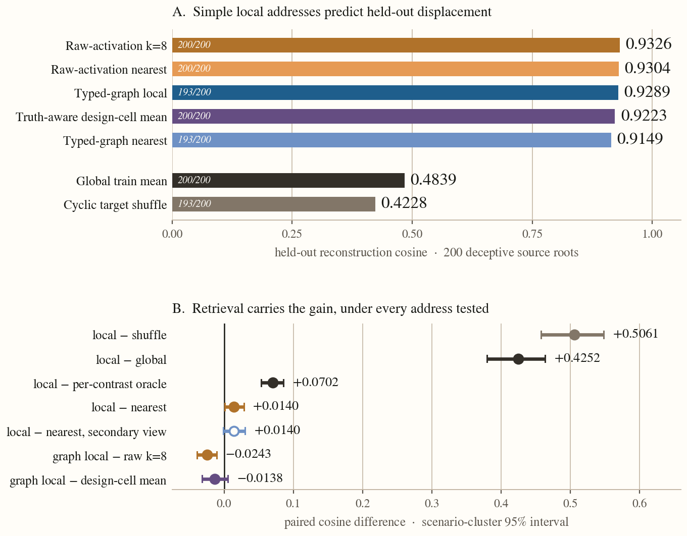
The typed-graph local estimator beats its global direction by +0.4252 [+0.3799, +0.4638], the largest gap measured in this program. Its sign-flipped prediction lands near −0.93, an orientation sanity check showing that the reconstruction is consistently directed rather than benefiting from unsigned similarity.
The twist: the address is coarse and simple
I built the first estimator on a typed relational graph using residual streams, attention rows, and typed metadata. The registered simple-address diagnostic then asked whether that machinery was necessary.
It was not. Euclidean nearest neighbors on raw activations do as well or better (0.9304–0.9326). Within the typed-graph estimator, averaging its neighborhood adds only +0.0140 over its graph-nearest exemplar (0.9289 versus 0.9149). Retrieval, not graph structure or elaborate aggregation, carries almost all of the gain.
A mean over the design cell—turn, intervention history, pressure exposure, and true status—also reaches 0.9223. This is a privileged truth-aware explanatory baseline, not a deployable controller. It locates what the address recovers.
Restricted to its own design cell, the activation-nearest exemplar does not beat the cell mean (−0.0022, interval crossing zero). On all 195 covered queries, the unrestricted nearest neighbor already falls inside the query’s cell. The result is therefore coarse addressability: activation similarity recovers the design-cell partition. At the available support, it does not detectably order targets within that cell.
Most of the motion is generic
Two controls ask how specifically this organization belongs to deceptive-to-honest transitions:
- an unoriented estimator built from all same-truth transitions reaches 0.9060;
- a nuisance shuffle that preserves the design-cell target distribution while destroying exact source–target pairing reaches 0.9175.
Finding 2 · Specificity
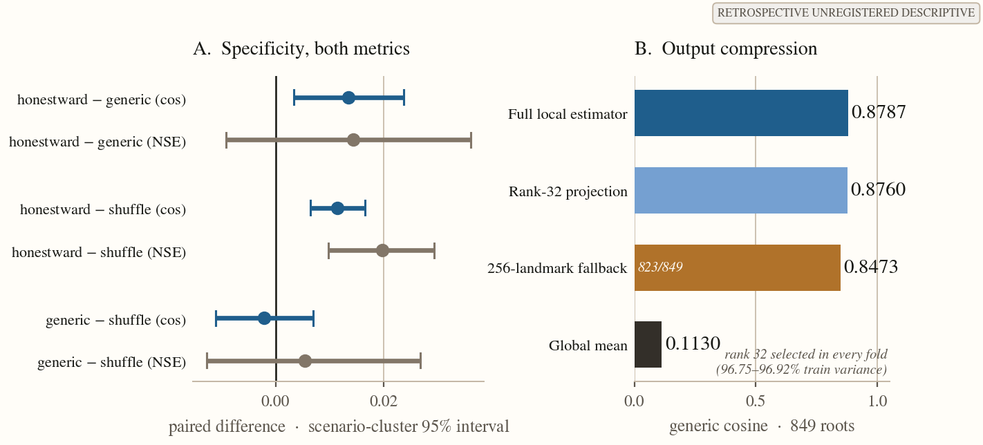
Most of the motion is generic; the remaining margins are small
Aggregate reconstruction gives orientation. Paired intervals decide the comparisons.
Aggregate reconstruction
These aggregate means are not arithmetic substitutes for the paired margins.
Honestward over generic motion
+0.0135cosine · CI above zero +0.0144normalized error · CI crosses zero metric-dependentExact pairing over cell shuffle
+0.0114cosine · CI above zero +0.0198normalized error · CI above zero positive on both metricsOpen paired intervals
| Comparison | Cosine margin | Normalized-error margin |
|---|---|---|
| Honestward over generic motion | +0.0135 [+0.0034, +0.0237] | +0.0144 [−0.0091, +0.0362] metric-dependent |
| Exact pairing over nuisance shuffle | +0.0114 [+0.0064, +0.0166] | +0.0198 [+0.0097, +0.0293] both positive |
Most of what the address retrieves is generic, design-conditioned transition organization. The honestward advantage over generic motion is small and metric-dependent: positive in cosine, with the normalized-error interval crossing zero. The exact-pairing advantage over the nuisance shuffle is also small, but positive on both reported metrics.
The vocabulary is compact and partially factorized
Finding 3 · Representation
A compact output vocabulary, with a destination-conditioned rule
Compression describes the outputs. Factorization describes how to construct them.
Output compression
96.75–96.92% of training variance retained in every fold.
Destination-conditioned factorization
Desired status and destination program are supplied.
Output compactness. A rank-32 projection preserves the full estimator almost exactly (0.8760 versus 0.8787 across 849 roots). A tested 256-landmark compression of the source-side address book misses its frozen target. That scheme was insufficient; other source-side representations remain open.
Specificity + compression audit
Small directional residue, compact output space
Paired intervals and the frozen compression frontier.
Destination-conditioned factorization. The symbolic descriptor receives the requested transition, desired status, and destination program. With that destination supplied, action alone reaches 0.6808; adding the source state lifts reconstruction to 0.8915, positive in all five held-out-family folds. Endpoint subtraction explains 66.3% of the observed lift; a learned source coupling supplies the remaining +0.0710.
Factorization audit
Source coordinates add beyond endpoint subtraction
Five held-out-family folds; fold consistency, not a confidence interval.
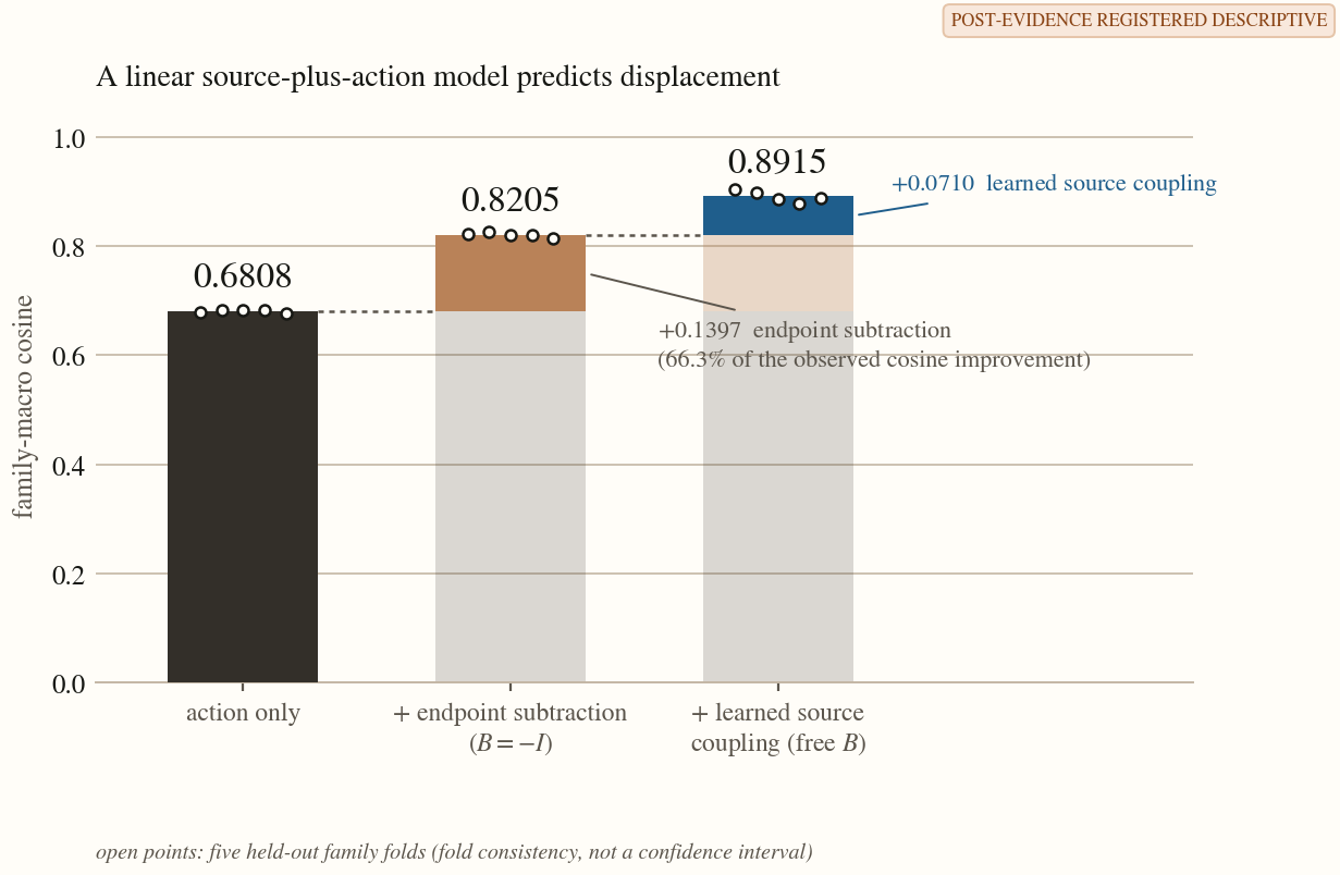
The displacement vocabulary is therefore partially a linear function of what destination was requested and where the model was. This is a compact target constructor, not a target-free predictor.
From reconstruction to control
0.9326 cosine
not yet tested
The earlier experiments draw the boundary:
Capability ledger
The information budget changes at every rung
These are different estimands, not one leaderboard.
| Capability | Instrument | Result | Verdict |
|---|---|---|---|
| Supplied-target actuation | Fixed-dose steering; target given | 591/600 fixes, 0 honest harms | Works given target |
| Target-free prose control | Prospective L16 controller | Net 0.0000; forced firing −0.083 | Refuted |
| Pre-commitment warning | Three instruments; truth-aware comparators | AUROCs 0.42 / 0.37; geometry −0.022 | Utility bound |
| Post-commitment readout | Raw-residual probe | Brier 0.0015; wins 20/20 families | Nearly linear |
| Cross-construction transfer | Zero-shot readout | 0.51–0.63 versus native 0.78–0.87 | Weak; cause unknown |
| Causal displacement injection | Matched controls | Not run | Open |
Actuation works when the corrective target is supplied and fails in the one prospective test where the controller had to find a target itself. Inferring the destination remains the unsolved step. The reconstructed displacement has not yet crossed the separate prediction-to- intervention boundary.
What I think this means
The first study said: reading is linear, control is selection. This one adds a third clause: the transition is coarsely addressable. Nearby source activations retrieve displacement examples that transfer across held-out families with the simplest possible lookup.
The controls make the claim more useful, not weaker. The gain is retrieval rather than graph machinery. The design cell explains most of the address. The deception-specific residue is small. A rank-32 output space and a destination-conditioned source-plus-action model make the next causal test concrete.
Take a retrieved or predicted displacement, inject it under matched random, sign-flipped, global-direction, and no-intervention controls, then re-decode behavior. If it works, the address becomes a handle. If it fails, reconstruction and intervention separate cleanly. Either outcome resolves the next question.
The pre-status activation is a coarse address into a compact, mostly generic displacement vocabulary. The decisive next experiment is whether that address becomes a causal handle.
The registry, compact evidence receipts, figure producers, tests, and scientific code are public at github.com/rajarshighoshal/deception-pressure-geometry.
If you think I got something wrong, I’d like to hear it.
GPU compute was supported by a BlueDot Impact Rapid Grant.